Getting started
This page shows how to get started with PyMDE for four common tasks:
visualizing datasets in two or three dimensions;
generating feature vectors for supervised learning;
computing classical embeddings, like PCA and spectral embedding;
drawing graphs in 2 or 3 dimensions;
Note
To learn how to create custom embeddings (with custom objective functions and constraints), sanity check embeddings, identify possible outliers in the original data, embed new data, and more, see the MDE guide. (We recommend reading the getting started guide first.)
What is an embedding?
An embedding of a finite set of items (such as biological cells, images, words, nodes in a graph, or any other abstract object) is an assignment of each item to a vector of fixed length; the original items are embedded or mapped into a real vector space. The length of the vectors is called the embedding dimension. An embedding is represented concretely by a matrix, in which each row is the embedding vector of an item.
Embeddings provide concrete numerical representations of abstract items, for use in downstream computational tasks. For example, when the embedding dimension is 2 or 3, embeddings can be used to create a sort of chart or atlas of the items. In such a chart, each point corresponds to an item, and its coordinates in space are given by the embedding vector. These visualizations can help scientists and analysts identify patterns or anomalies in the original data, and more generally make it easier to explore large collections of data. PyMDE can embed into 2 or 3 dimensions, but it can also be used to embed into many more dimensions, which is useful when generating features for machine learning tasks.
For an embedding to be useful, it must be faithful to the original data (the items) in some way. To make it easy to get started, PyMDE provides two high-level functions for creating embeddings, based on related but different notions of faithfulness. These functions handle the common case in which each item is associated with either an original high-dimensional vector or a node in a graph. The functions are
The first creates embeddings that focus on the local structure of the data, putting similar items near each other and dissimilar items not near each other. The second focuses more on the global structure, choosing embedding vectors to respect some notion of original distance or dissimilarity between items.
We’ll see how to use these functions below.
Visualizing data
When the embedding dimension is 2 (or 3), embeddings can be used to visualize large collections of items. These visualizations can sometimes lead to new insights into the data.
Preserving neighbors
Let’s create an embedding that preserves the local structure
of some data, using the pymde.preserve_neighbors function. This function
is based on on preserving the k-nearest neighbors of each original vector
(where k is a parameter that by default is chosen on your behalf).
We’ll use the MNIST dataset, which contains images of handwritten digits, as an example. The original items are the images, and each item (image) is represented by an original vector containing the pixel values.
import pymde

mnist = pymde.datasets.MNIST()
Next, we embed.
mde = pymde.preserve_neighbors(mnist.data, verbose=True)
embedding = mde.embed(verbose=True)
The first argument to preserve_neighbors is the data matrix: there are
70,000 images, each represented by a vector of length 784 , so mnist.data
is a torch.Tensor of shape (70,000, 784). The optional keyword argument
verbose=True flag turns on helpful messages about what the function is
doing. The embedding dimension is 2 by default.
The function returns a pymde.MDE object, which can be thought of as
describing the kind of embedding we would like. To compute the embedding, we
call the embed method of the mde object. This returns a
torch.Tensor of shape (70,000, 2), in which embedding[k] is
the embedding vector assigned to the image mnist.data[k].
We can visualize the embedding with a scatter plot. In the scatter plot, we’ll color each point by the digit represented by the underlying image.
pymde.plot(embedding, color_by=mnist.attributes['digits'])
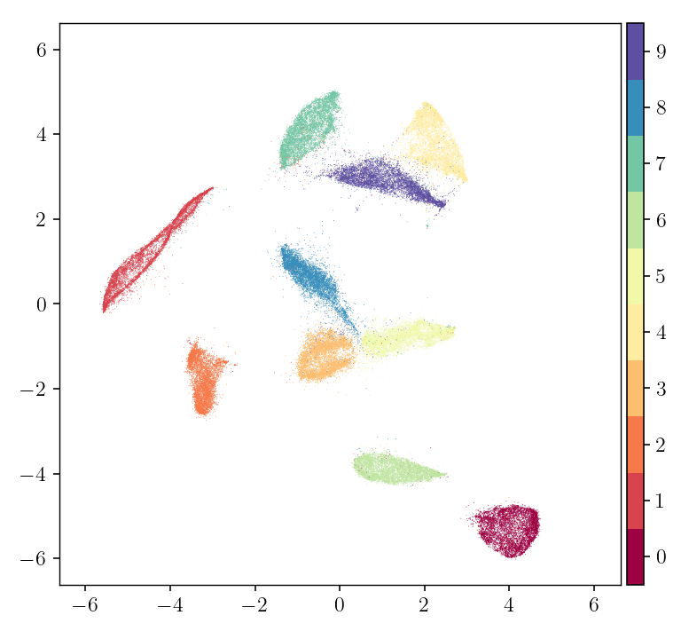
We can see that similar images are near each other in the embedding, while dissimilar images are not.
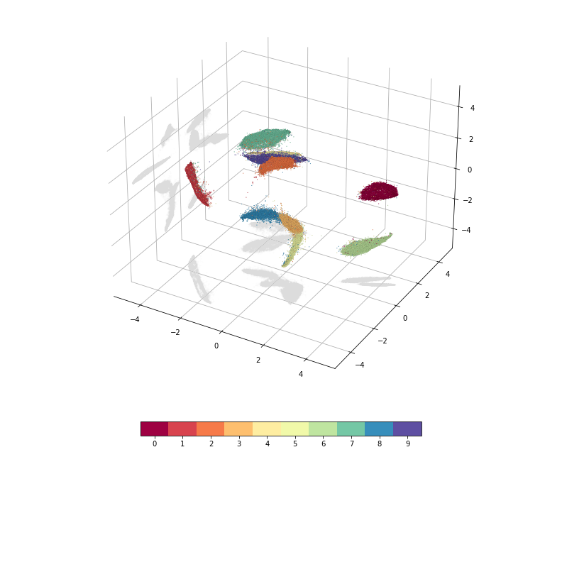
It is also possible to embed into three or more dimensions. Here is an example with three dimensions.
mde = pymde.preserve_neighbors(mnist.data, embedding_dim=3, verbose=True)
embedding = mde.embed(verbose=True)
pymde.plot(embedding, color_by=mnist.attributes['digits'])
Customizing embeddings
The pymde.preserve_neighbors function takes a few keyword arguments
that can be used to customize the embedding. For example, you
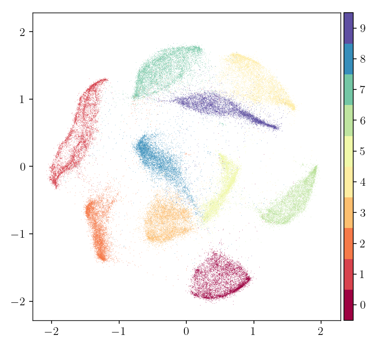
can impose a pymde.Standardized constraint: this
causes the embedding to have uncorrelated columns, and prevents it from
spreading out too much.
embedding = pymde.preserve_neighbors(mnist.data, constraint=pymde.Standardized()).embed()
pymde.plot(embedding, color_by=mnist.attributes['digits'])
To learn about the other keyword arguments, read the tutorial on MDE, then consult the API documentation.
For more in-depth examples of creating neighborhood-based visualizations, including 3D embeddings, see the MNIST and single-cell genomics example notebooks.
Accessing the underlying graph
You can access the graph underlying the MDE problem returned by
pymde.preserve_neighbors, using the following code.
edges = mde.edges
weights = mde.distortion_function.weights
The value weights[i] is the weight for the edge edges[i].
Preserving distances
Next, we’ll create an embedding that roughly preserves the global structure of some original data, by preserving some known original distances between some pairs of items. We will embed the nodes of an unweighted graph. For the original distance between two nodes, we’ll use the length of the shortest path connecting them.
The specific graph we’ll use is an academic coauthorship graph, from Google Scholar: the nodes are authors (with h-index at least 50), and two authors have an edge between them if either has listed the author as a coauthor.
import pymde
import torch

device = 'cuda' if torch.cuda.is_available() else 'cpu'
google_scholar = pymde.datasets.google_scholar()
mde = pymde.preserve_distances(google_scholar.data, device=device, verbose=True)
embedding = mde.embed()
The data attribute of the google_scholar dataset is a
pymde.Graph object, which encodes the coauthorship network.
The pymde.preserve_distances function returns a pymde.MDE
object, and calling the embed method computes the embedding.
Notice that we passed in a device to pymde.preserve_distances;
this embedding approximately preserves over 80 million distances, so using a
GPU can speed things up.
Next we plot the embedding, coloring each point by how many coauthors the author has in the network (normalized to be a percentile).
pymde.plot(embedding, color_by=google_scholar.attributes['coauthors'])
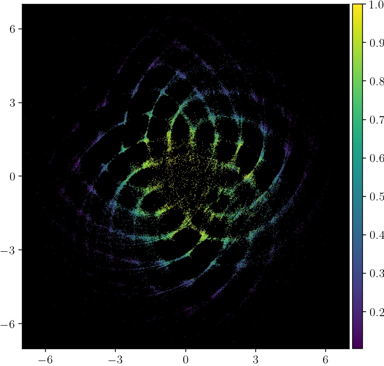
The most collaborative authors are near the embedding, and less collaborative ones are on the fringe. It also turns out that the diameter of the embedding is close to the true diameter of the graph.
For a more in-depth study of this example, see the notebook on Google Scholar.
Customizing embeddings
The pymde.preserve_distances function takes a few keyword arguments
that can be used to customize the embedding.
To learn about the keyword arguments, read the tutorial on MDE, then consult the API documentation.
Accessing the underlying graph
You can access the graph underlying the MDE problem returned by
pymde.preserve_distances, using the following code.
edges = mde.edges
distances = mde.distortion_function.deviations
The value distances[i] is the weight (which should be interpreted as a
distance) for the edge edges[i].
Plotting
Scatter plots
The pymde.plot function can be used to plot embeddings with dimension
at most 3. It takes an embedding as the argument, as well a number of optional
keyword arguments. For example, to plot an embedding and color each point
by some attribute, use:
pymde.plot(embedding, color_by=attribute)
The attribute variable is a NumPy array of length embedding.shape[0],
in which attribute[k] is a tag or numerical value associated with item k.
For example, in the MNIST data, each entry in attribute is an int
between 0 and 9 representing the digit depicted in the image;
for single-cell data, each entry might be a string describing the type of
cell. Typically the attribute is not used to create the embedding, so coloring
by it is a sanity-check that the embedding has preserved prior knowledge about
the original data.
This function can be configured with a number of keyword arguments, which can
be seen in the API documentation.
Movies
The pymde.MDE.play method can be used to create an animated GIF of the
embedding process. To create a GIF, first call pymde.MDE.embed with
the snapshot_every keyword argument, then call play:
mde.embed(snapshot_every=1)
mde.play(savepath='/path/to/file.gif')
The snapshot_every=1 keyword argument instructs the MDE object to
take a snapshot of the embedding during every iteration of the solution
algorithm. The play method generates the GIF, and saves it to savepath.
This method can be configured with a number of keyword arguments,
which can be seen in the API documentation.
Generating feature vectors
The embeddings made via pymde.preserve_neighbors and
pymde.preserve_distances can be used as feature vectors for supervised
learning tasks. You can choose the dimension of the vectors by specifying the
embedding_dim keyword argument, e.g.,
embedding = pymde.preserve_neighbors(data, embedding_dim=50).embed()
Classical embeddings
PyMDE provides a few implementations of classical embeddings, for convenience.
To produce a PCA embedding of a data matrix, use the pymde.pca
method, which returns an embedding:
embedding = pymde.pca(data_matrix, embedding_dim)
To create a Laplacian embedding based on the nearest neighbors of each row in a
data matrix or each node in a graph, use the pymde.laplacian_embedding
method, which returns an MDE problem:
mde = pymde.laplacian_embedding(data, embedding_dim, verbose=True)
embedding = mde.embed()
To create a spectral embedding based on a sequence of edges (a torch.Tensor
of shape (n_edges, 2)) and weights, use pymde.quadratic.spectral.
(These embeddings are called “quadratic embeddings” in the MDE monograph.)
Drawing graphs
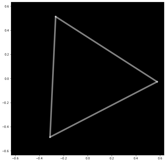
PyMDE can be used to draw graphs in 2 or 3 dimensions. Here is a very simple example that draws a cycle graph on 3 nodes.
edges = torch.tensor([
         [0, 1],
         [0, 2],
         [1, 2]
])
triangle = pymde.Graph.from_edges(edges)
triangle.draw()
Here is a more interesting example, which embeds a ternary tree. The tree is created using the NetworkX package.
import networkx

ternary_tree = networkx.balanced_tree(3, 6)
graph = pymde.Graph(networkx.adjacency_matrix(ternary_tree))
embedding = graph.draw()
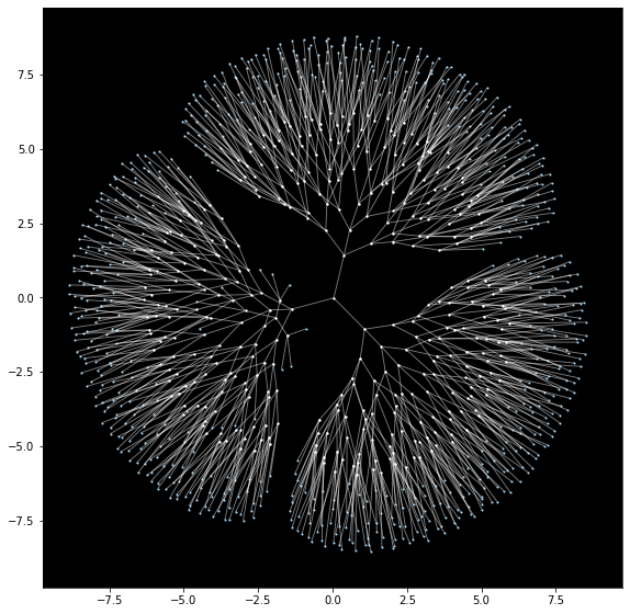
On a standard CPU, it takes PyMDE just 2 seconds to compute this layout; for comparison, it takes NetworkX 30 seconds to compute a similar layout.
You can embed into 3 dimensions by passing embedding_dim=3 to the draw
method.
For more in-depth examples, see the notebook on drawing graphs,
and the API documentation of pymde.Graph.
Using a GPU
If you have a CUDA-enabled GPU, you can use it to speed up the optimization routine which computes the embedding.
The functions pymde.preserve_neighbors and
pymde.preserve_distances, as well as the method Graph.draw, all take a
keyword argument, called device, which controls whether or not a GPU is
used. Pass device='cuda' to use your GPU. (PyMDE computes embeddings on CPU
by default.)
For example, the below code shows how to create a neighbor-preserving embedding of MNIST using a GPU.
import pymde

mnist = pymde.datasets.MNIST()
mde = pymde.preserve_neighbors(mnist.data, device='cuda', verbose=True)
embedding = mde.embed(verbose=True)
On an NVIDIA GeForce GTX 1070, the embed method took just 5 seconds.
Reproducibility
PyMDE’s optimization algorithm does not rely on randomness. However,
some functions, such as pymde.preserve_neighbors, may use random sampling
when generating the edges for an MDE problem. This means that if you call
pymde.preserve_neighbors multiple times on the same data set, you might
obtain slightly different MDE problems and therefore slightly different
embeddings. To prevent this from happening, you can set random seed state via
the pymde.seed function.
For example, the following code block will always create the same embedding.
import pymde

mnist = pymde.datasets.MNIST()

pymde.seed(0)
mde = pymde.preserve_neighbors(mnist.data, verbose=True)
embedding = mde.embed(verbose=True)