MDE
The central concept in PyMDE is the Minimum-Distortion Embedding (MDE) problem. An MDE problem is an optimization problem whose solution is an embedding.
We can interpret an MDE problem as a declarative description of the properties
an embedding should satisfy. MDE problems in PyMDE are represented by
the pymde.MDE object.
In this part of the tutorial, we explain what an MDE problem is. Then we
show how to construct MDE problems using PyMDE, with custom objective
functions and constraints. We also describe some of the useful methods that
the pymde.MDE class provides, and how to sanity-check and compare
embeddings.
The MDE framework
In this section, we introduce the concept of an MDE problem, whose solution is an embedding. At a high-level, the objective of an MDE problem is to minimally distort known relationships between some pairs of items, while possibly satisfying some constraints.
We first explain this abstractly. In the next section, we show how to make MDE problems using PyMDE.
Embedding matrix
An MDE problem starts with a set \(\mathcal{V}\) of \(n\) items, \(\mathcal{V} = \{0, 1, ..., n - 1\}\). An embedding of the set of items is a matrix \(X \in \mathbf{R}^{n \times m}\), where \(m\) is the embedding dimension. The rows of \(X\) are denoted \(x_0, x_1, \ldots, x_{n-1}\), with \(x_i\) being the embedding vector associated with item \(i\). The quality of an embedding will depend only on the Euclidean distances between the embedding vectors,
Distortion functions
We make our preferences on the \(d_{ij}\) concrete with distortion functions associated with the edges. These have the form
where \(\mathcal E\) is a set of edges \((i , j)\), with \(0 \leq i < j < n\). This set of edges may contain all pairs, or a subset of pairs, but it must be non-empty.
For convenience, we can assume the edges are listed in some fixed order, and label them as 1, 2, ldots, p, where \(p = |\mathcal E|\). We can then represent the collection of distortion functions as a single vector distortion function \(f : \mathbf{R}^p \to \mathbf{R}^p\), where \(p = |\mathcal E|\) and \(f_k\) is the distortion function associated with the \(k\)-th edge.
Distortion functions are usually derived either from weights, or from
original distances or deviations between some pairs of items. PyMDE
provides a library of both types of distortion functions, in
pymde.penalties and pymde.losses.
Distortion functions from weights
We start with nonzero weights \(w_1, w_2, \ldots, w_p\), one for each edge. A positive weight means the items in the edge are similar, and a negative weight means they are disimilar. The larger the weight is, the more similar the items are; the more negative the weight, the more dissimilar.
A vector distortion function \(f : \mathbf{R}^{p} \to \mathbf{R}^p\) derived from weights has component functions
where \(w_k\) is a scalar weight and \(p_{\text{attractive}}\) and \(p_{\text{repulsive}}\) are penalty functions. Penalty functions are increasing functions: the attractive penalty encourages the distances to be small, while the repulsive penalty encourages them to be large, or at least. not small.
Attractive penalties are 0 when the input is 0, and grow otherwise. The attractive and repulsive penalties can be the same, e.g. they can both be quadratics \(d \mapsto d^2\), or they can be different. Typically, though, repulsive penalties go to negative infinity as the input approaches 0, and to 0 as the input grows large.
Distortion functions from deviations
A vector distortion function \(f : \mathbf{R}^{p} \to \mathbf{R}^p\) derived from original deviations has component functions
where \(\ell\) is a loss function, and \(\delta_k\) is a scalar deviation or dissimilarity score associated with the \(k\)-th edge.
The deviations can be interpreted as targets for the embedding distances: the loss function is 0 when \(d_k = \delta_k\), and positive otherwise. So a deviation \(\delta_k`\) of 0 means that the items in the k-th edge are the same, and the larger the deviation, the more dissimilar the items are.
The simplest example of a loss function is the squared loss
Average distortion
The value \(f_{ij}(d_{ij})\) is the distortion associated for the pair \((i, j) \in \mathcal E\). The smaller the distortion, the better the embedding captures the relationship between \(i\) and \(j\).
The goal is to minimize the average distortion of the embedding X, defined as
possibly subject to the constraint that \(X \in \mathcal X\), where \(\mathcal X\) is a set of permissible embeddings. This gives the optimization problem
This optimization problem is called an MDE problem. Its solution is the embedding.
Constraints
We can optionally impose constraints on the embedding.
For example, we can enforce the embedding vectors to be standardized, which means that they are centered and identity covariance, that is, \((1/n) X^T X = I\). When a standardization constraint is imposed, the embedding problem always has a solution. Additionally, the standardization constraint forces the embedding to spread out. When using distortion functions from weights, this means we do not need repulsive penalties (but can choose to include them anyway).
Or, we can anchor or pin some of the embedding vectors to fixed values.
Constructing an MDE problem
In PyMDE, instances of the pymde.MDE class are MDE problems. The
pymde.preserve_neighbors and pymde.preserve_distances
functions we saw in the previous part of the tutorial both returned
MDE instances.
To create an MDE instance, we need to specify five things:
the number of items;
the embedding dimension;
the list of edges (a
torch.Tensor, of shape(n_edges, 2))the vector distortion function; and
an optional constraint.
Let’s walk through a very simple example.
Items
Let’s say we have five items. In PyMDE, items are represented by consecutive integer labels, in our case 0, 1, 2, 3, and 4.
Edges
Say we know that item 0 is similar to items 1 and 4, 1 is similar to 2, 2 is similar to 3, and 3 is similar to 4. We include these pairs in a list of edges
edges = torch.tensor([[0, 1], [0, 4], [1, 2], [2, 3]])
Distortion function
Next, we need to encode the fact that each edge represents some degree of similarity between the items it contains. We’ll use a quadratic penalty \(f_k(d_k) = w_k d_k^2\) (other choices are possible). We’ll associate a weight 1 to the first edge, 2 to the second edge, 5 to the third edge, and 6 to the fourth edge; this conveys that 0 is somewhat similar to 1 but more similar to 4, 2 is yet more similar to 3, and 3 is yet more similar to 4. We write this in PyMDE as
weights = torch.tensor([1., 2., 5., 6.])
f = pymde.penalties.Quadratic(weights)
Constraint
The last thing to specify is the constraint. Since we’re using a distortion function based on only positive weights, we’ll need a standardization constraint.
constraint = pymde.Standardized()
Construction
We can now construct the MDE problem:
import pymde

mde = pymde.MDE(
  n_items=5,
  embedding_dim=2,
  edges=edges,
  distortion_function=f,
  constraint=pymde.Standardized())
The mde object represents the MDE problem whose goal is to minimize
the average distortion with respect to f, subject to the standardization
constraint. This object can be thought of describing the kind of embedding
we would like.
Embedding
To obtain the embedding, we call the pymde.MDE.embed method:
embedding = mde.embed()
print(embedding)
tensor([[ 0.0894, -1.8689],
        [-0.7726, -0.1450],
        [-0.6687,  0.5428],
        [-0.5557,  0.9696],
        [ 1.9077,  0.5015]])
We can check that the embedding is standardized with the following code:
print(embedding.mean(axis=0))
print((1/mde.n_items)*embedding.T @ embedding)
tensor([4.7684e-08, 5.9605e-08])
tensor([[1.0000e+00, 7.4506e-08],
        [7.4506e-08, 1.0000e+00]])
We can also evaluate the average distortion:
print(mde.average_distortion(embedding))
tensor(6.2884)
Summary
This very simple example showed all the components required to construct an MDE problem. The full documentation for the MDE class is available in the API documentation.
In the next section, we’ll learn more about distortion functions and how to create them.
Distortion functions
A distortion function is just a Python callable that maps the embedding distances to distortions, using PyTorch operations. Its call signature should be
torch.Tensor(shape=(n_edges,), dtype=torch.float) -> torch.Tensor(shape=(n_edges,), dtype=torch.float)
For example, the quadratic penalty we used previously can be implemented as
weights = torch.tensor([1., 2., 5., 6.]
def f(distances):
  return weights * distances.pow(2)
A quadratic penalty based on original deviations could be implemented as
deviations = torch.tensor([1., 2., 5., 6.]
def f(distances):
  return (distances - deviations).pow(2)
In many applications, you won’t need to implement your own distortion functions. Instead, you can choose one from a library of useful distortion functions that PyMDE provides.
PyMDE provides two types of distortion functions: penalties, which are based on weights, and losses, based on original deviations. (A natural question is: Where do the weights or original deviations come from? We’ll see some recipes for creating edges and their weights / deviations in the next part of the tutorial, which covers preprocessing.)
Penalties
Penalties: distortion functions derived from weights.
A vector distortion function \(f : \mathbf{R}^{p} \to \mathbf{R}^p\) derived from weights has component functions
where \(w_k\) is a scalar weight, \(p\) is a penalty function, and \(d_k\) is an embedding distance. The penalty encourages distances to be small when the weights are positive, and encourages them to be not small when the weights are negative.
When an MDE problem calls a distortion function, \(d_k\) is the Euclidean distance between the items paired by the \(k\)-th edge, so \(w_k\) should be the weight associated with the \(k\)-th edge, and \(f_k(d_k)\) is the distortion associated with the edge.
Every penalty can be used with positive or negative weights. When \(w_k\) is positive, \(f_k\) is attractive, meaning it encourages the embedding distances to be small; when \(w_k\) is negative, \(f_k\) is repulsive, meaning it encourages the distances to be large. Some penalties are better suited to attracting points, while others are better suited to repelling them.
Negative weights. For negative weights, it is recommended to only use one of the following penalties:
pymde.penalties.Log
pymde.penalties.InvPower
pymde.penalties.LogRatio
These penalties go to negative infinity as the input approaches zero, and to zero as the input approaches infinity. With a negative weight, that means the distortion function goes to infinity at 0, and to 0 at infinity.
Using other penalties with negative weights is possible, but it can lead to pathological MDE problems if you are not careful.
Positive weights. Penalties that work well in attracting points are those that are \(0\) when the distance is \(0\), grows when the distance is larger than \(0\). All the penalties in this module, other than the ones listed above (and the function described below), can be safely used with attractive penalties. Some examples inlcude:
pymde.penalties.Log1p
pymde.penalties.Linear
pymde.penalties.Quadratic
pymde.penalties.Cubic
pymde.penalties.Huber
Combining penalties.
The PushAndPull function can be used to combine two penalties, an attractive
penalty for use with positive weights, and a repulsive penalty for use with
negative weights. This leads to a distortion function of the form
For example:
weights = torch.tensor([1., 1., -1., 1., -1.])
attractive_penalty = pymde.penalties.Log1p
repulsive_penalty = pymde.penalties.Log

distortion_function = pymde.PushAndPull(
    weights,
    attractive_penalty,
    repulsive_penalty)
Example. Distortion functions are created in a vectorized or elementwise fashion. The constructor takes a sequence (torch.Tensor) of weights, returning a callable object. The object takes a sequence of distances of the same length as the weights, and returns a sequence of distortions, one for each distance.
For example:
weights = torch.tensor([1., 2., 3.])
f = pymde.penalties.Quadratic(weights)

distances = torch.tensor([2., 1., 4.])
distortions = f(distances)
# the distortions are 1 * 2**2 == 4, 2 * 1**2 == 2, 3 * 4**2 = 48
print(distortions)
prints
torch.tensor([4., 2., 48.])
Losses
Losses: distortion functions derived from original deviations.
A vector distortion function \(f : \mathbf{R}^{p} \to \mathbf{R}^p\) derived from original deviations has component functions
where \(\ell\) is a loss function, \(\delta_k\) is a nonnegative deviation or dissimilarity score, \(d_k\) is an embedding distance,
When an MDE problem calls a distortion function, \(d_k\) is the Euclidean distance between the items paired by the k-th edge, so \(\delta_k\) should be the original deviation associated with the k-th edge, and \(f_k(d_k)\) is the distortion associated with the edge.
The deviations can be interpreted as targets for the embedding distances: the loss function is 0 when \(d_k = \delta_k\), and positive otherwise. So a deviation \(\delta_k`\) of 0 means that the items in the k-th edge are the same, and the larger the deviation, the more dissimilar the items are.
Distortion functions are created in a vectorized or elementwise fashion. The constructor takes a sequence (torch.Tensor) of deviations (target distances), returning a callable object. The object takes a sequence of distances of the same length as the weights, and returns a sequence of distortions, one for each distance.
Some examples of losses inlcude:
pymde.losses.Absolute
pymde.losses.Quadratic
pymde.losses.SoftFractional
Example.
deviations = torch.tensor([1., 2., 3.])
f = pymde.losses.Quadratic(deviations)

distances = torch.tensor([2., 5., 4.])
distortions = f(distances)
# the distortions are (2 - 1)**2 == 1, (5 - 2)**2 == 9, (4 - 3)**2 == 1
print(distortions)
prints
torch.tensor([1., 9., 1.])
Constraints
PyMDE currently provides three constraint sets:
pymde.Centered, which constrains the embedding vectors to have mean zero;pymde.Standardized, which constrains the embedding vectors to have identity covariance (and have mean zero);pymde.Anchored, which pins specific items (called anchors) to specific values (i.e., this is an equality constraint on a subset of the embedding vectors).
Centered
If a constraint is not specified, the embedding will be centered, but no other restrictions will be placed on it. Centering is without loss of generality, since translating all the points does not affect the average distortion.
To explicitly create a centering constraint, use
constraint = pymde.Centered()
Standardized
The standardization constraint is
where \(n\) is the number of items (i.e., the number of rows in \(X\)) and \(\mathbf{1}\) is the all-ones vector.
A standardization constraint can be created with
constraint = pymde.Standardized()
The standardization constraint has several implications.
It forces the embedding to spread out.
It constrains sum of embedding distances to have a root-mean-square value of \(\sqrt{(2nm)/(n-1)}\), where \(m\) is the embedding dimension. We call this value the natural length of the embedding.
It makes the columns of the embedding uncorrelated, which can be useful if the embedding is to be used as features in a supervised learning task.
When the distortion function is based on penalties and all the weights are positive, you must impose a standardization constraint, which will force the embedding to spread out. When the weights are not all positive, a standardization constraint is not required, but is recommended: MDE problems with standardization constraints always have a solution. Without the constraint, problems can sometimes be pathological.
When the distortion functions are based on losses, care must be taken to ensure that the original deviations and embedding distances are on the same scale. This can be done by rescaling the original deviations to have RMS equal to the natural length.
Anchored
The anchor constraint is
where \(\text{anchors}\) is a subset of the items and \(v_i\) is a concrete value to which \(x_i\) should be pinned.
An anchor constraint can be created with
# anchors holds the item numbers that should be pinned
anchors = torch.tensor([0., 1., 3.])
# the ith row of values is the value v_i for the ith item in anchors
values = torch.tensor([
  [0., 0.],
  [1., 2.],
  [-1., -1.],
])
constraint = pymde.Anchored(anchors, values)
Below is a GIF showing the creation of an embedding of a binary tree, in which the leaves have been anchored to lie on a circle with radius 20.
See this notebook for the code to make this embedding (and GIF).
Custom constraints
It is possible to specify a custom constraint set. To learn how to do so, consult the API documentation.
Computing embeddings
After creating an MDE problem, you can compute an embedding by calling
the its embed method. The embed method takes
a few optional hyper-parameters. Here is its documentation.
- MDE.embed(X=None, eps=1e-05, max_iter=300, memory_size=10, verbose=False, print_every=None, snapshot_every=None)
Compute an embedding.
This method stores the embedding in the
Xattribute of the problem instance (mde.X). Summary statistics related to the fitting process are stored insolve_stats(mde.solve_stats).All arguments have sensible default values, so in most cases, it suffices to just type
mde.embed()ormde.embed(verbose=True)- Parameters:
X (torch.Tensor, optional) – Initial iterate, of shape
(n_items, embedding_dim). When None, the initial iterate is chosen randomly (and projected onto the constraints); otherwise, the initial iterate should satisfy the constraints.eps (float) – Residual norm threshold; quit when the residual norm is smaller than
eps.max_iter (int) – Maximum number of iterations.
memory_size (int) – The quasi-Newton memory. Larger values may lead to more stable behavior, but will increase the amount of time each iteration takes.
verbose (bool) – Whether to print verbose output.
print_every (int, optional) – Print verbose output every
print_everyiterations.snapshot_every (int, optional) – Snapshot embedding every
snapshot_everyiterations; snapshots saved as CPU tensors toself.solve_stats.snapshots. If you want to generate an animation with theplaymethod after embedding, setsnapshot_everyto a positive integer (like 1 or 5).
- Returns:
The embedding, of shape
(n_items, embedding_dim).- Return type:
torch.Tensor
Computing an embedding saves some statistics in the
solve_stats attribute.
Sanity-checking embeddings
The MDE framework gives you a few ways to sanity-check embeddings.
Plotting embeddings
If your embedding is in three or fewer dimensions, the first thing to do
(after calling the embed method) is to simply plot it with pymde.plot,
and color it by some attributes that were not used in the embedding process.
You can optionally pass in a list of edges to this function, which will
superimpose edges onto the scatter plot. Read the API documentation for
more details.
GIFs can be created with the pymde.MDE.play method.
The CDF of distortions
Regardless of the embedding dimension, the next thing to do is to
plot the cumulative distribution function (CDF) of distortions. You can
do this by calling the distortions_cdf method on an MDE instance:
mde.distortions_cdf()
This will result in a plot like
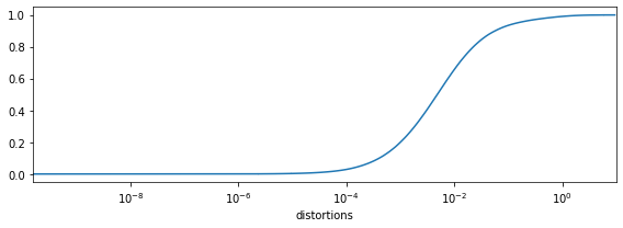
In this particular case, we see that most distortions are very small, but roughly 10 percent of them are much larger. This means that embedding the items was “easy”, except for these 10 percent of edges.
Outliers
Next, you should manually inspect the items in, say, the 10 most highly distorted pairs; this is similar to debugging a supervised learning model by examining its mistakes. You can get the list of edges sorted from most distorted to least like so:
pairs, distortions = mde.high_distortion_pairs().
highly_distorted_pairs = pairs[:10]
In the case of a specific embedding of MNIST, some of these pairs ended up containing oddly written digits, while others looked like they shouldn’t have been paired:
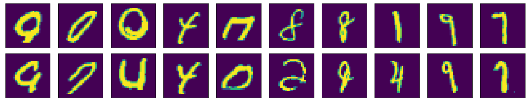
After inspecting the highly distorted pairs, you have a few options. You can leave your embedding as is, if you think your embedding is reasonable; you can throw out some of the highly distorted edges if you think they don’t belong; you can modify your distortion functions to be less sensitive to large distances; or you can even remove some items from your original dataset, if they appear malformed.
Comparing embeddings
Suppose you want to compare two different embeddings, which have the same
number of items and the same embedding dimension. If you have an MDE instance,
you can evaluate the average distortion of each embedding by calling
its average_distortion method.
It can also be meaningful to compute a distance between two embeddings. The average distortion is invariant to rotations and reflections of embeddings, so two embeddings must first be aligned before they can be compared.
To align one embedding to another, use the pymde.align function:
aligned_embedding = pymde.align(source=embedding, target=another_embedding)
This function rotates and reflects the source embedding to be as close to the target embedding as possible, and returns this rotated embedding. After aligning, you can compare embeddings by plotting them (if the dimension is 3 or less), or by computing the Frobenius norm of their difference (this distance will make sense if both embeddings are standardized, since that will put them on the same scale, but it will make less sense otherwise).
Embedding new points
Suppose we have embedded some number of items, and later we obtain additional items of the same type that we wish to embed. For example, we might have embedded the MNIST dataset, and later we obtain more images we’d like to embed.
Often we want to embed the new items without changing the vectors for the old data. To do so, we can solve a small MDE problem involving the new items and some of the old ones: some edges will be between new items, and importantly some edges will connect the new items to old items. The old items can be held in place with an anchor constraint.
For example, here is how to update an embedding of MNIST.
import pymde
import torch

mnist = pymde.datasets.MNIST()

n_train = 35000
train_data = mnist.data[:n_train]
val_data = mnist.data[n_train:]

train_embedding = pymde.preserve_neighbors(
    train_data, verbose=True).embed(verbose=True)
updated_embedding = pymde.preserve_neighbors(
    torch.vstack([train_data, val_data]),
    constraint=pymde.Anchored(torch.arange(n_train), train_embedding),
    verbose=True).embed(verbose=True)
A complete example is provided in the below notebook.